A shared latent space for operator learning
A neural operator learns the solution operator of a partial differential equation from data. Most parameterizations reduce a discretized function to a reduced space with an encoder, approximate the target there with a processor, and reconstruct it in the physical space with a decoder. In nonlinear architectures the encoder and the decoder are fitted to the data of a single task, so the labels must serve both the physics and the representation of functions, and little of the representation survives a change of equation, geometry, discretization or modality.
Daedalus separates the two problems, as self-supervised pre-training did for language and vision. A task-agnostic functional autoencoder (FAE) is pre-trained on synthetic analytic functions that belong to no equation, and the reduced space it induces is frozen and reused. Since the pretext distribution is engineered rather than sampled from one physics, a single space serves functions of different origin, geometry, discretization and modality, which is what the paper means by a universal latent space. The labels of a downstream problem then serve the physics alone.
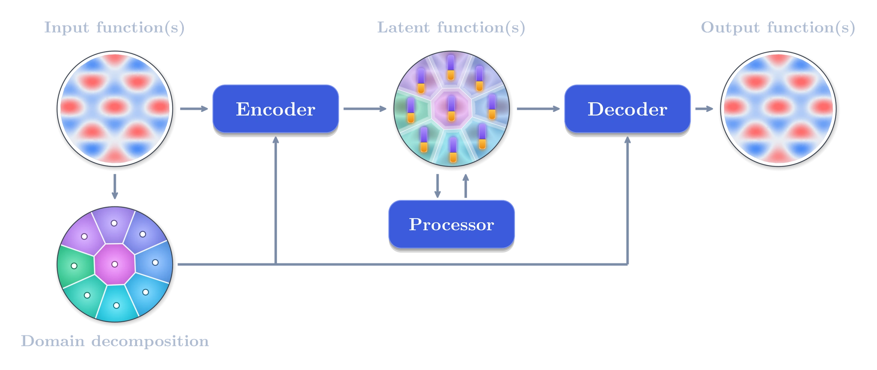
Two ingredients make such a representation transferable: a decomposition of the domain, so that an unfamiliar global field becomes a collection of local ones, and a normalization of every partition into a common frame, which removes its position, size and amplitude from what is learned. Both are described below, together with the remaining components of the method.
Scalar functions on point clouds
The FAE works on one scalar function at a time, given as values at points whose number and placement are arbitrary. A velocity field, a multi-variable state or the colors of a photograph are encoded one channel at a time, so the representation is agnostic to what the values mean. The encoder reduces the points to an embedding, and the decoder returns the value of the function at any coordinate, so the cloud a field is observed on and the cloud it is reconstructed on are independent.
Decomposition into partitions Read more about partitioning →
A single embedding per function would be a bottleneck of fixed size, for a smooth field and a finely structured one alike. Daedalus therefore cuts the cloud into P partitions by a fast k-means clustering of the coordinates, recomputed for every input, encodes every partition with the same encoder, and answers a query from the partitions that cover it. Partitions may overlap slightly across their boundaries. Since more partitions mean smaller neighborhoods, the partition count sets the resolution of the representation, and it is chosen after training, per input and per task.
Partition normalization Read more about partition normalization →
Before a partition is encoded, partition normalization (PartNorm) carries it into a common frame. Its points are shifted to their center cp and scaled by their extent sp into the box [−1, 1]2, and its values are mapped onto [−1, 1] by their mid-range μp and half-range σp. The encoder sees only the normalized partition and describes its shape, the morphologic embedding ζm,p, while the frame itself is kept aside as the static features ζs,p and replayed exactly by the decoder.
This has two consequences. Partitions that are similar after normalization receive nearly the same embedding whatever field they come from, so the model needs to have seen partitions of a similar shape rather than fields of the same physical kind. The encode-decode map is also exactly equivariant to translation, dilation, value shift and value scaling, which affect only the frame.
The encoder and the latent hypersphere Read more about the functional autoencoder →
The encoder lifts the points of a partition and averages them, which makes it indifferent to their number and order, and then refines one embedding through many units. After every unit the embedding is returned to a fixed length, so every morphologic embedding is a direction on a hypersphere in dζ dimensions. Each update is first stripped of its component along the current embedding, so the embedding turns along the sphere rather than growing or shrinking. The units are re-applied with shared weights, which makes the encoder deep without making it large.
The decoder as a neural field Read more about derivatives →
The decoder is a conditional neural field. For a query point it reads the embedding of a partition that contains it and the coordinate of the query in that partition's frame, and returns the value there, mapped back through the frame. Nothing is computed across queries, so a field can be decoded at the encoded points, on a finer grid, or where nothing was observed.
The same property makes the decoded field differentiable at little cost. The decoder is a composition of smooth layers, so the field it returns on a partition is a smooth function of position rather than a set of values at points, and its spatial derivatives follow exactly from automatic differentiation. Since the value at one query depends on no other query, the Jacobian of all decoded values with respect to their coordinates has no entries between different points, and one forward-mode pass per coordinate axis returns the derivative along that axis at every point at once, each pass costing little more than a decoding, with neither finite differences nor the full Jacobian.
Training on synthetic functions
The backbone never sees a PDE solution. Every batch is drawn on the fly from analytic distributions on the unit disk, radial sines with a few modes for both backbones of the paper, with no dataset and no solver. Generation needs no storage, never repeats a function, and leaves the distribution fully controlled. Two backbones are trained this way: a 128-dimensional analysis backbone, behind the analyses and the demos of this site, and an 8-dimensional operator-learning backbone, far cheaper for training operators.
The effective spatial frequency Read more about the effective spatial frequency →
A model trained on smooth sines also represents shocks and photographs, because it never sees a whole field, only normalized partitions, and a small partition of a complicated field appears simple once it is magnified to fill the frame. The paper measures this with the effective spatial frequency of a partition, how quickly the slope of the normalized field changes across it. Measured in this way, the family of a function matters little. The errors of twelve unrelated families collapse onto one curve of the effective frequency, and more partitions bring any field into the training band.
Generalization to physical fields Read more about reconstruction →
Trained on radial sines on a disk, the analysis backbone reconstructs fields from real physics datasets, compressible flows with shocks and shear layers, an acoustic wave, an incompressible flow, and the displacement and stresses of elastic bodies with holes, as well as 48 photographs, one color channel at a time. The error decreases steadily with the partition count. The same model also accepts functions sampled on curves and completes partially observed fields with plausible functions of its training family.
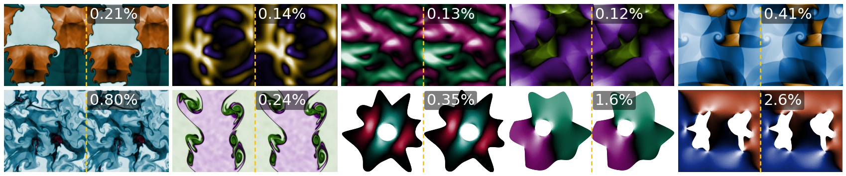
The limitations follow from the training band. A partition whose effective frequency stays outside it is not represented accurately, a partition needs enough points, and where nothing is observed the completion follows the training functions.
Operator learning in the latent space Read more about operator learning →
Freezing the encoder and the decoder makes caching possible. The embeddings of a training set are computed once, and an operator, a transformer over the partition embeddings called the processor, trains on stored embeddings without touching the points. A training step then costs the processor alone, whatever the resolution of the data, and a short cooldown on decoded fields closes most of the gap that training on embeddings leaves. Against GAOT and RIGNO-12, two state-of-the-art end-to-end frameworks, on 28 problems under one protocol:
On one RTX 4090 (24 GB), with variable geometry and the partitioning included.
The memory measured on one RTX 4090 grows affinely with the partitions and the processor depth. It is extrapolated to 768 GB, 32 times one RTX 4090, assuming that the memory is pooled by sharding the model and the batch across the eight cards.
Why this changes the scale of operator learning
At a fixed compute budget, these measurements change the scale at which foundation models for physics can be pre-trained and fine-tuned, and at which models for a single task can be trained from scratch.
- Pre-training. End-to-end pre-training passes every step through the encoder and the decoder of the full point cloud, so its cost grows with the resolution of the data and dense corpora are downsampled to fit. On cached embeddings a step costs the processor alone at any resolution, so the same budget pre-trains a far larger processor on data kept at full resolution, and a single node of eight GPUs reaches the projected scale above.
- Fine-tuning. A pre-trained processor adapted to a new task reads the same frozen representation, so it fine-tunes on cached embeddings of the new data on a single consumer GPU rather than on the hardware that pre-trained it.
- Models trained from scratch. A model for one task, trained on one consumer GPU, handles problems of millions of points, 64 times larger than end-to-end training fits there, and trains up to 13.6 times faster, so a large model trains in a few hours rather than days.