Operator learning

Operators on a frozen latent space

Daedalus separates learning what functions look like from learning the physics. Its functional autoencoder (FAE) is pre-trained once on synthetic analytic functions, with no labels and no solver, and then frozen. An operator is learned on the partition embeddings, entirely inside the reduced space, so the labels of a downstream problem pay only for the physics. What reaches the operator is a small collection of embeddings rather than a point cloud, so the discretization of the field stays outside the operator.

A single backbone, trained once, serves every downstream task. Since no task trains it further, a new operator incurs no additional cost for the backbone, and the cost of a task is that of its processor alone.

All operators of the paper, and all operator results reported here, use the operator-learning backbone, whose embeddings have d_ζ = 8 dimensions.

Problem setting

An operator maps input fields to output fields and is learned from pairs of them. The backbone encodes one scalar channel at a time, so a vector field or a set of fields is reduced channel by channel on the same partitions. The following terms are used throughout.

Processor

The trainable network. It maps the embeddings of the input fields, one per partition, to embeddings of the output fields on the same partitions.

Input and target embeddings

The encodings of the input fields of a training pair and of its target fields, on the same partitions.

Frozen or unfrozen

The encoder and the decoder keep their pre-trained weights, or they are unfrozen and trained together with the processor, which fine-tunes the backbone on the task at hand.

Physical loss

Evaluated on fields. The output embeddings are decoded at the points of the target and compared with it.

Latent loss

Evaluated on embeddings. The output embeddings are compared with the target embeddings, and nothing is decoded.

Input and output cache

With a frozen backbone, the partitions and input embeddings of the training set are computed once and stored, and under the latent loss the target embeddings as well.

Three training modes follow. The end-to-end mode partitions, encodes, processes and decodes at every step, the physical mode skips the first two with an input cache, and the latent mode runs the processor alone. An unfrozen backbone changes its embeddings at every step, so it trains uncached and on the physical loss only.

The processor

The processor is a transformer over the partition embeddings that refines its tokens with the on-sphere update of the encoder. Every update is orthogonalized against the current embedding and applied under a learned scale, which discards the component that a normalization would undo. The attention reads the relative positions of the partitions through two-dimensional rotary position embeddings, and for a time-continuous operator every unit is conditioned on the lead time by feature-wise linear modulation (FiLM). In the performance measurements it has a width of 512, eight heads, two units applied four times each, and 3.69 million parameters (3.79 million with the encoder and the decoder), in bf16 mixed precision.

Two choices keep the attention affordable over thousands of partitions. The grouping orders the embeddings along a randomly rotated Z-order curve and concatenates every run of M consecutive embeddings, a compact group of neighbors, into one token, so the attention runs over T = P/M tokens while the projections and the feed-forward layer mix the members of a group locally. The windowed attention permutes the tokens at random, cuts them into W windows and attends within each, which lowers the cost of one application from O(T²) to O(T²/W). Every window is spread over the whole cloud, so the attention stays global, the windows are redrawn at every application of a unit, and every block draws a new curve, so the groups slide across depth.

The transformer is one admissible processor among several. The embeddings are anchored at the partition centers and form a point cloud of their own, so any map from such a set to a set of the same kind can serve, a graph neural network over the centers being a natural alternative. With the backbone frozen and the embeddings cached, the processor can be exchanged without retraining the FAE.

Latent and physical losses

A partition is decoded in its normalized frame and returned to physical values by its value frame, a shift and a scale. In the FAE this frame is the one the encoder stored, and it is exact. A processor predicts it together with the morphology, so an error in a predicted frame shifts or rescales the whole partition.

The physical loss decodes the prediction at the points of the target and takes the relative L¹ error per function and output channel, averaged over a batch, so every channel counts equally whatever its amplitude. The latent loss compares the two parts of a predicted embedding with those of the encoded target separately,

ℒ_lat = (ℒ_m + w_s ℒ_s) / (1 + w_s),   ℒ_m = 𝔼[1 − cos(ζ̂_m, ζ_m)],   ℒ_s = 𝔼[log₂(1 + ‖ζ̂_s − ζ_s‖ / ‖ζ_s‖)],

with w_s = 0.3. The morphologic term is a cosine distance between directions on the sphere, which ignores the magnitude of an embedding. The static term is the relative error of the predicted static features, compressed by the logarithm. Of these features the processor predicts the value frames, while the geometry frame is copied from the input. Both terms equal one at the uninformative baseline, so w_s is a genuine relative weight.

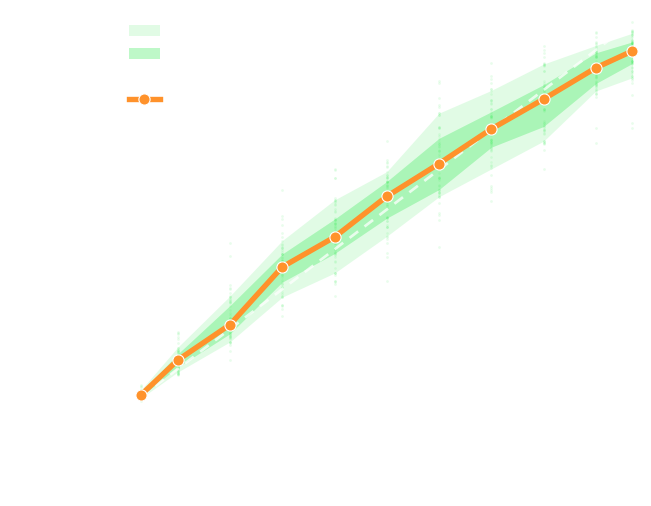
The latent loss stands in for the physical error only as far as nearby embeddings decode to nearby fields. A functional autoencoder can reconstruct accurately and still fail this, and a processor that matches its embeddings would then optimize something only loosely related to the field it predicts. This property can be measured directly.

Input and output caching

With the backbone frozen, the partitioner, the encoder and the decoder are fixed maps, so whatever they compute from the training data alone can be computed once and stored. The backward pass already skips the frozen encoder, since no trainable parameter precedes it, so an input cache saves the time of the partitioning and of the encoding with little change in memory. The output cache stores the encoded targets as well, and the decoder leaves the step together with its backward pass.

Removing the decoder matters most for memory, although it is the shallower of the two maps. It lies between the processor and a physical loss, so the backward pass runs through it and its activations are stored for every point of every partition, times its depth. The saving grows with the number of points, and it would matter most for three-dimensional problems, whose clouds are far larger at a comparable resolution.

The cache is written once into memory-mapped arrays on a local disk and read back by row, so the training set never has to fit into the host memory. It holds the input embeddings and, under the latent loss, the target embeddings, or under the physical loss the coordinates, assignments and target values that the decoder needs. Every function is partitioned once, whereas an uncached run draws a new partitioning at every visit.

Caching requires that the physical space be crossed exactly twice, once by the encoder and once by the decoder. For an architecture that never leaves the physical space, or returns to it at every layer, there is nothing to cache.

A physical cooldown

A run has up to three phases. A warmup on small batches raises the learning rate linearly, the main phase decays it along a cosine to a constant tail, and an optional cooldown closes the run at that tail rate. The warmup and the main phase train on the latent loss with both caches, where a step involves the processor alone. The cooldown, the final fifth of the epochs, switches to the physical loss, on an input cache built when it starts, so the total cost stays close to that of latent training.

The switch serves two purposes. First, it closes whatever gap the latent proxy leaves, since it optimizes the error itself. Second, it balances the static and the morphologic part of a prediction, which the latent loss weighs by the fixed w_s although their effect on the field differs from partition to partition. Independent errors in the predicted value frames leave a honeycomb pattern of partition-shaped cells, and the physical loss, which weighs each part by its actual effect, removes it.

Training on the physical loss from the start does not achieve the same result on every problem. PartNorm factors every decoded value into a predicted frame and a predicted morphology, so many combinations decode to nearly the same field, channels are coupled only through the processor, and nothing provides a residual connection in the physical space. An operator trained on the physical loss alone can therefore settle in a basin of lower quality. The cooldown switches only once the processor has reached the right basin.

The cooldown can also unfreeze the encoder and the decoder, which then get an optimizer of their own with fresh moment estimates and a correct bias correction. An unfrozen backbone is specialized to one task, and since only the decoded output is supervised, nothing keeps its encoder and decoder inverse to each other. The fine-tuned backbone is stored together with the processor.

Accuracy benchmark

The paper compares the operator on the frozen backbone with two baselines trained end to end, GAOT and RIGNO-12, on 28 problems (RIGNO-12, the most expensive to train, on 24 of them). All three run through one data pipeline, with the same inputs, targets, splits, rollout and metric, and are otherwise free in their architecture, loss and training.

The problems cover incompressible flow (IEU, four families of initial conditions), compressible flow (CEU, five problems on 128² grids and a Rayleigh–Taylor instability under gravity, and the same five problems on their native 512² grids), acoustic waves (AWA), the Helmholtz equation (HEL), the Poisson equation (POI), the static equilibrium of linear and hyperelastic bodies (SEQ), and steady compressible flow past a body: three airfoils (NACA0012, NACA2412 and RAE2822, their shape perturbed from sample to sample) and ten bluff bodies, with the free-stream Mach number and angle of attack and the distance to the body as inputs and the density as output. The grid problems share one geometry across their samples, whereas the five elasticity problems and the four steady compressible flows are point clouds whose geometry changes from sample to sample.

The first 128 samples of a dataset form its test split and the next 128, or 96 for the Rayleigh–Taylor problem, its validation split, and between 1024 and 8192 samples follow for training. A time-dependent problem keeps every second snapshot up to the time index 14, or 10 for the Rayleigh–Taylor problem, and its evaluation rolls out from the initial snapshot in blocks of eight time indices and scores the final snapshot only. The error of a sample is the relative L¹ error of each output channel on the raw fields, averaged over the channels, and the reported value is its median over the test samples, at the checkpoint with the lowest validation median of the relative L² error. The total training time (TTT) is measured on four RTX 4090 cards, data loading and cache building included, and for Daedalus it excludes the pre-training of the backbone, which serves all 28 problems.

Accuracy and training cost

Daedalus is more accurate than GAOT on 23 of the 28 problems and more accurate than RIGNO-12 on all 24 on which it is trained. Averaged over the problems, the per-problem error of GAOT exceeds that of Daedalus by 23% and the error of RIGNO-12 by 265%, and their per-problem training times are 2.1 and 8.3 times longer. The error of GAOT is lower by more than 5% on four problems, IEU-VortexSheet, CEU-KH and CEU-RayleighTaylor on the 128² grids, and POI-Gauss. On the nine problems with a varying geometry, where GAOT cannot share its preprocessing across samples whereas cached embeddings remain available to Daedalus, the training time of GAOT is on average 2.7 times that of Daedalus and its error 30% higher. On the four steady compressible flows its error is higher on every problem, by 45% on average.

Four problems train faster with GAOT, by a factor of at most 1.2: CEU-RayleighTaylor (128²), CEU-BluffBody, HEL-Gauss and POI-Gauss. The fast mode of GAOT saves time only when every sample shares one geometry, whereas cached embeddings serve varying point clouds just as well.

Training regimes and the cost of freezing

The paper also trains the same processor in four regimes on eight of the problems, five evolution and three steady ones: on the latent loss throughout with both caches, on the physical loss throughout with the input cache, with the cooldown of the benchmark, and with an unfrozen cooldown that also trains the encoder and the decoder without a cache.

The physical loss lowers the error of the latent loss on every steady problem, by 33% in the geometric mean, but on the evolution problems its error is 22% higher, and 71% and 74% higher on AWA-Layer and CEU-Gauss (128²). Without the output cache it also takes 1.7 times as long to train. The cooldown avoids both drawbacks. On the steady problems it closes the proxy gap, with an error 31% below that of the latent loss and only 3% above that of the physical loss, and on the evolution problems it does no harm, its error being 8% below that of the latent loss, while it adds 16% to the training time.

The last regime quantifies how far the frozen space limits the operator. Unfreezing the backbone in the cooldown lowers the error of the frozen cooldown by a further 8% on the steady problems and does not help on the evolution problems, at 2.4 times the training time of the frozen cooldown, since an unfrozen backbone admits no cache. The gain costs the invertibility of the encoding and decoding and the interpretability of the embeddings, so the paper treats it as an option rather than the default.

Speed and memory

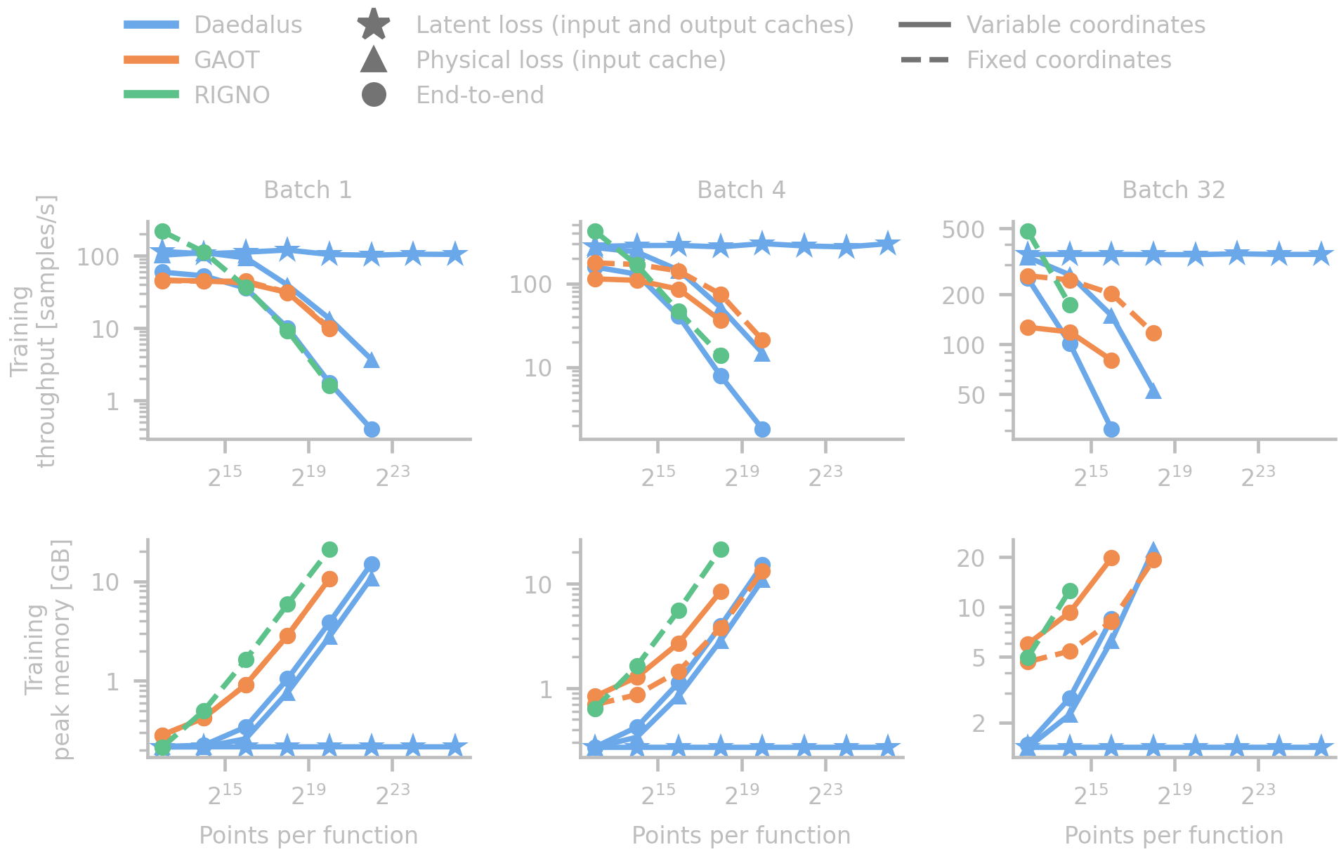
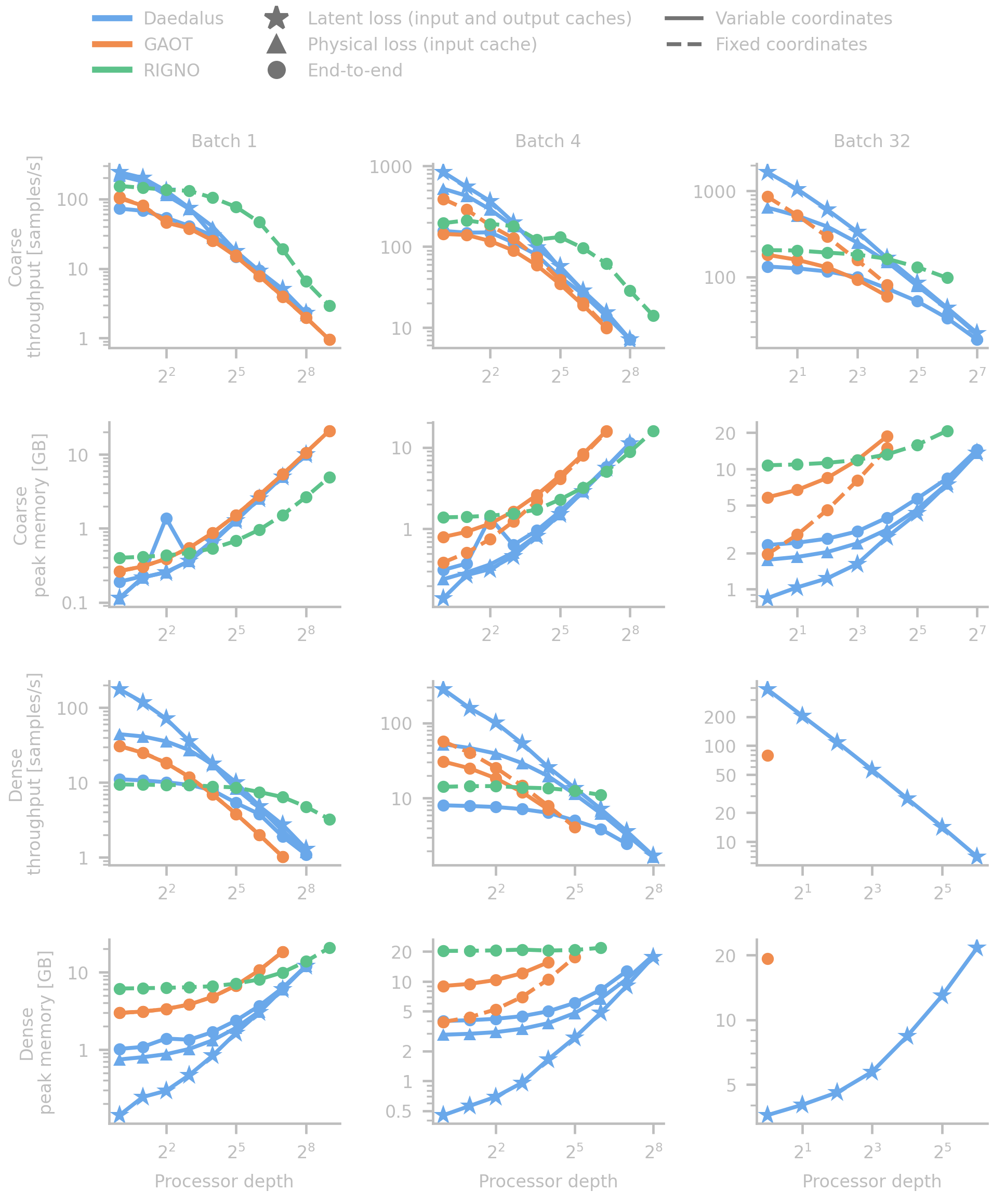
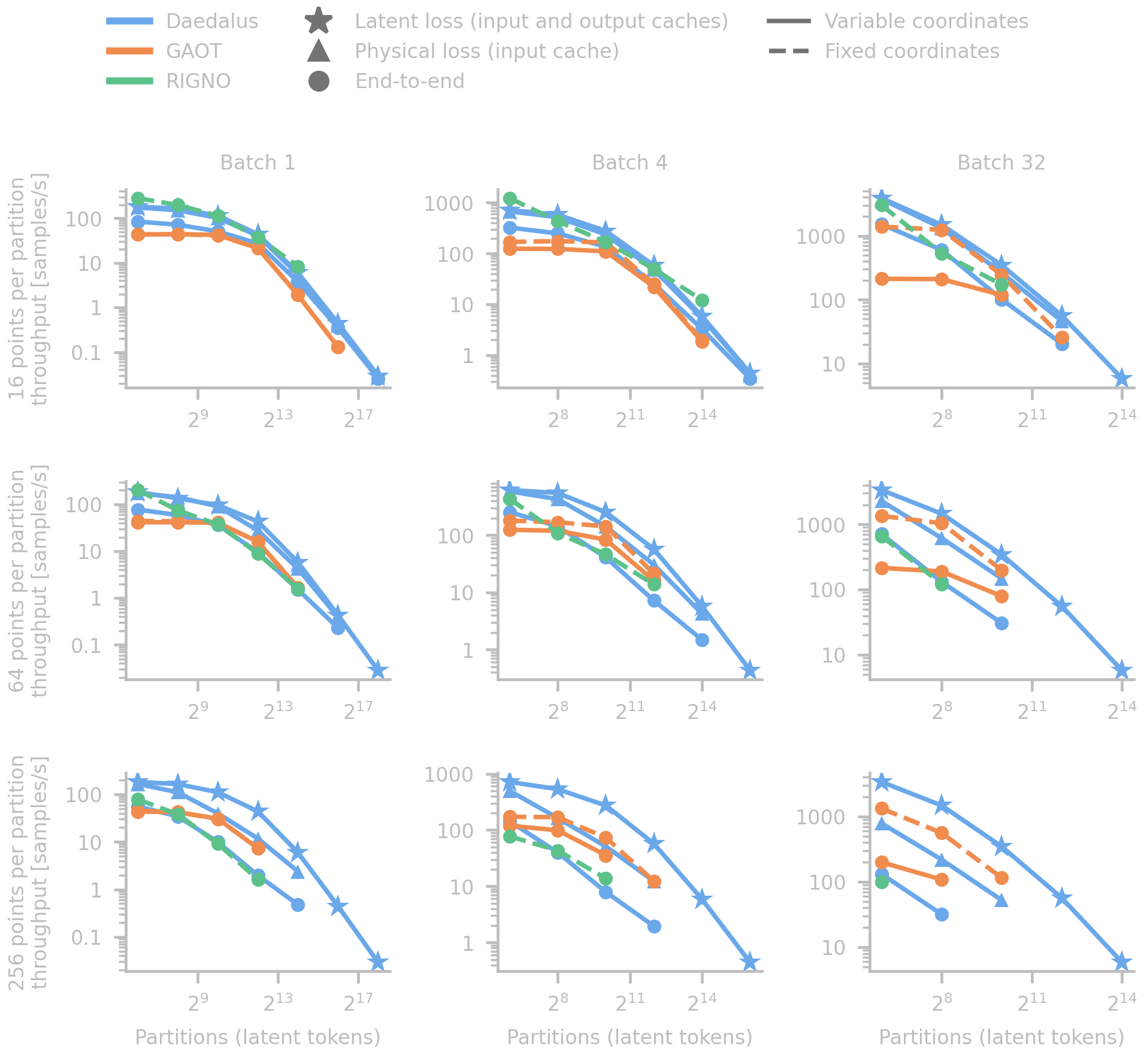
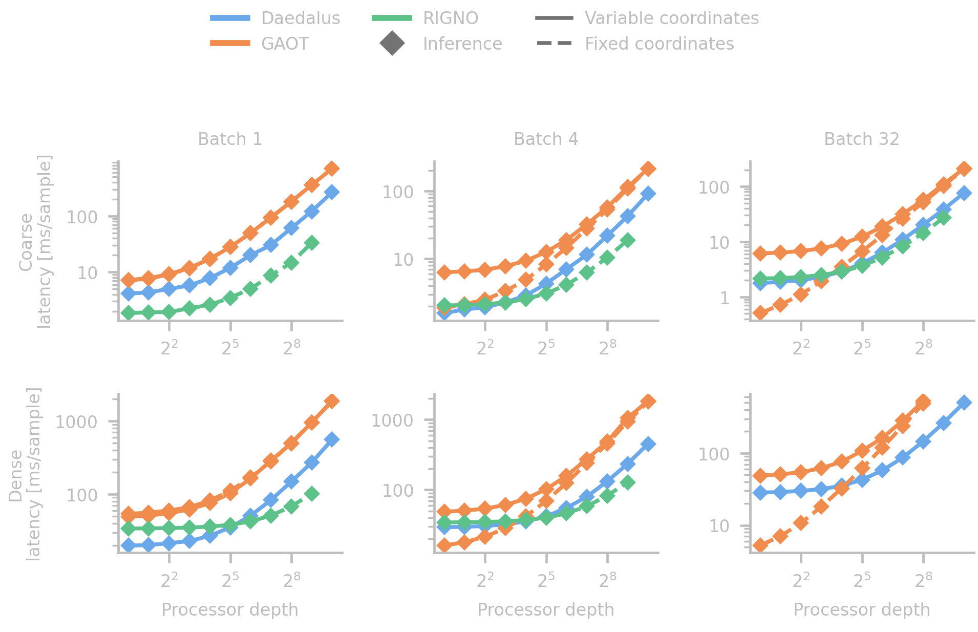
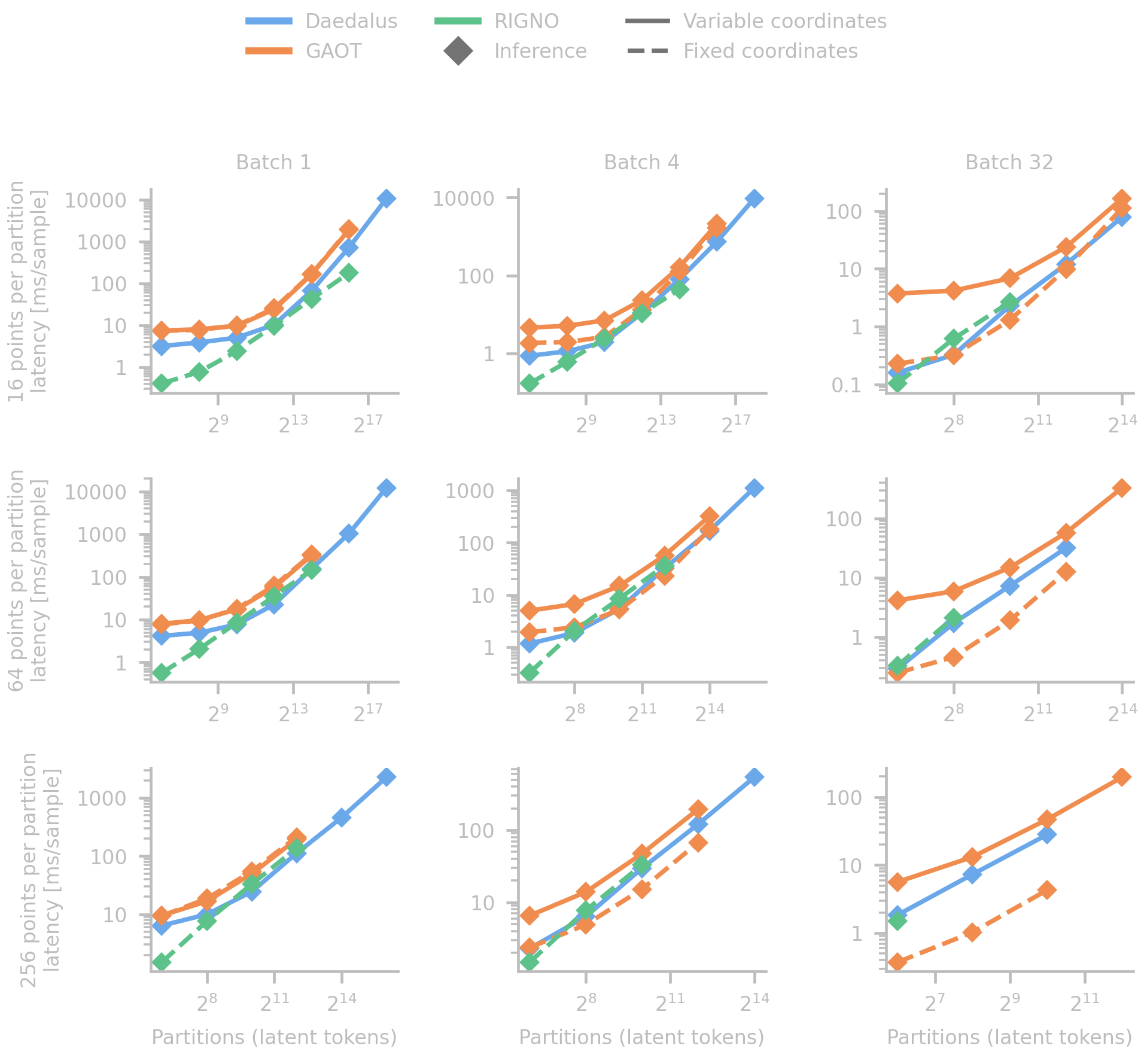
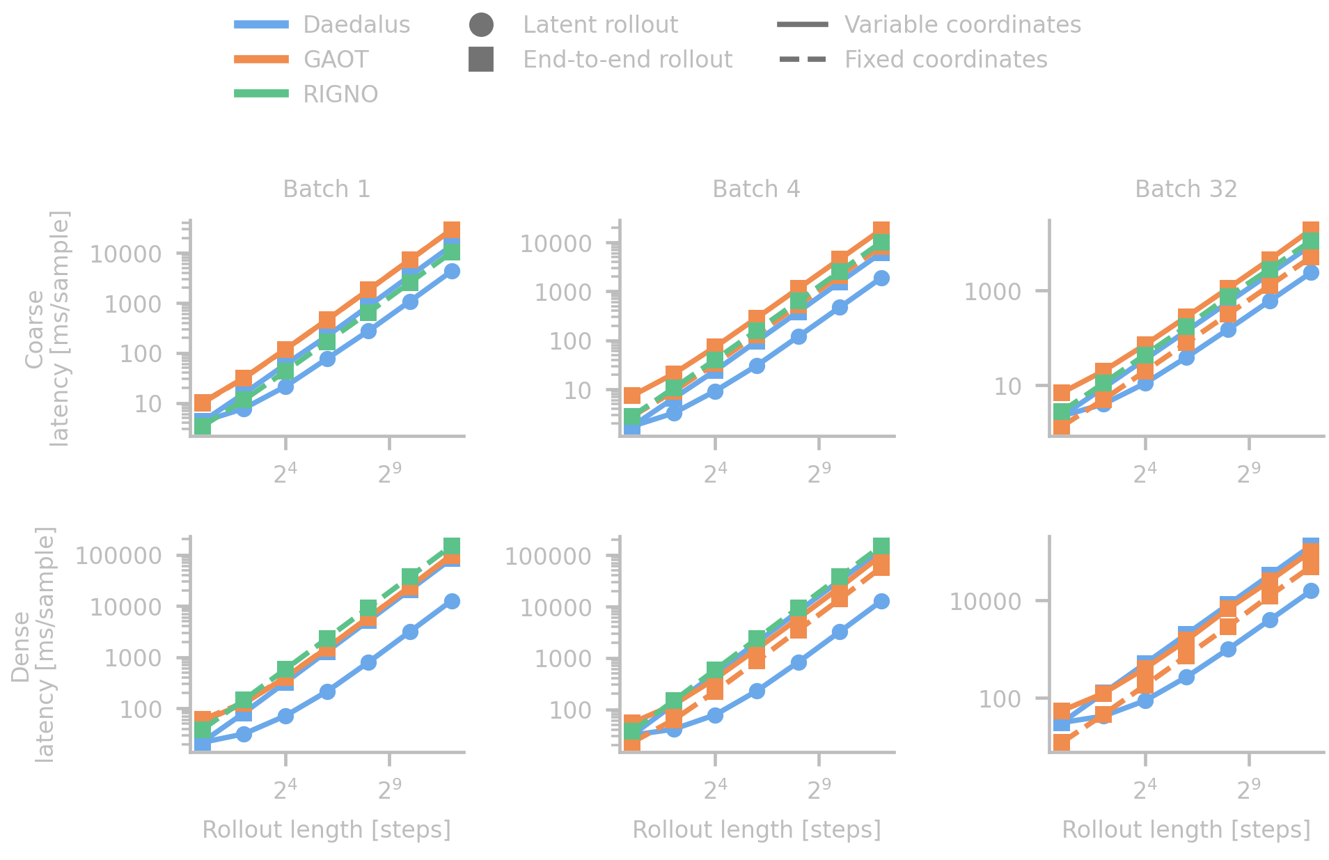
The performance benchmark times training and inference on synthetic problems of free size, with the same configurations, sweep points, protocol and functions for all three models and untrained weights, since the cost of a step does not depend on them. By default a function has 16384 points and 1024 partitions or latent tokens. Every measurement runs in a fresh process on one RTX 4090 with 24 GB.

The latent mode of Daedalus never touches the points, the physical mode runs the frozen decoder in every step, and the end-to-end mode partitions, encodes, processes and decodes at every step while training the backbone too. GAOT and RIGNO train end to end on graphs built before training. The depth counts the processor units of Daedalus, the transformer layers of GAOT and the message-passing steps of RIGNO, which hold about 1.6, 1.1 and 0.12 million parameters each.

On one RTX 4090 (24 GB), with variable geometry and the partitioning included.

The memory measured on one RTX 4090 grows affinely with the partitions and the processor depth. The projections extrapolate it to 768 GB, 32 times one RTX 4090, assuming that the memory is pooled by sharding the model and the batch across the eight cards.

Memory

The memory of the latent mode follows the processor alone, 0.22 GB at a batch of one and 1.41 GB at a batch of 32 for every space size, at least 13 times below any other setting from a million points on, and 49 times below GAOT at a million points and a batch of one. The physical mode keeps the encoder out of the step and needs 10.9 GB at 4.2 million points and a batch of one, against 15 GB end to end, while GAOT needs 10.6 GB and RIGNO 20.9 GB at a quarter of that size. Where a deep processor dominates, the three modes need about the same, and on the coarse problem at small batches RIGNO needs less than any of them.

Training throughput

The latent mode trains at about 105, 280 and 347 samples per second at batches of 1, 4 and 32 across all sizes, so dense training data need no downsampling. At a batch of one it is faster than GAOT with fixed coordinates by 1.2 to 2.7 times on the coarse problem and 2.4 to 5.7 times on the dense one, while against RIGNO the depth decides. When the number of partitions grows with the points, the latent and the physical mode train up to 18 times faster than GAOT on variable clouds.

Inference latency

At a batch of one, Daedalus infers faster than GAOT at every depth and partition count. At a batch of 32, GAOT with fixed coordinates is faster on shallow processors, until Daedalus overtakes it from 16 units on the coarse problem and 32 on the dense one. RIGNO is the fastest at large depth and on small problems, since its steps are small and its graph construction is not timed. At 1024 partitions, Daedalus infers on 16.8 million points in 2.5 seconds per sample.

Rollouts

A latent rollout starts flat, its cost dominated by the single encoding and decoding, and then grows linearly with a slope three to ten times smaller than that of an end-to-end rollout. At 4096 steps it is 6.6 to 10 times faster than the end-to-end rollout of Daedalus on the dense problem, and up to 9.6 times faster than GAOT and 12 times faster than RIGNO. No rollout grows in memory with its length.

Chunked inference

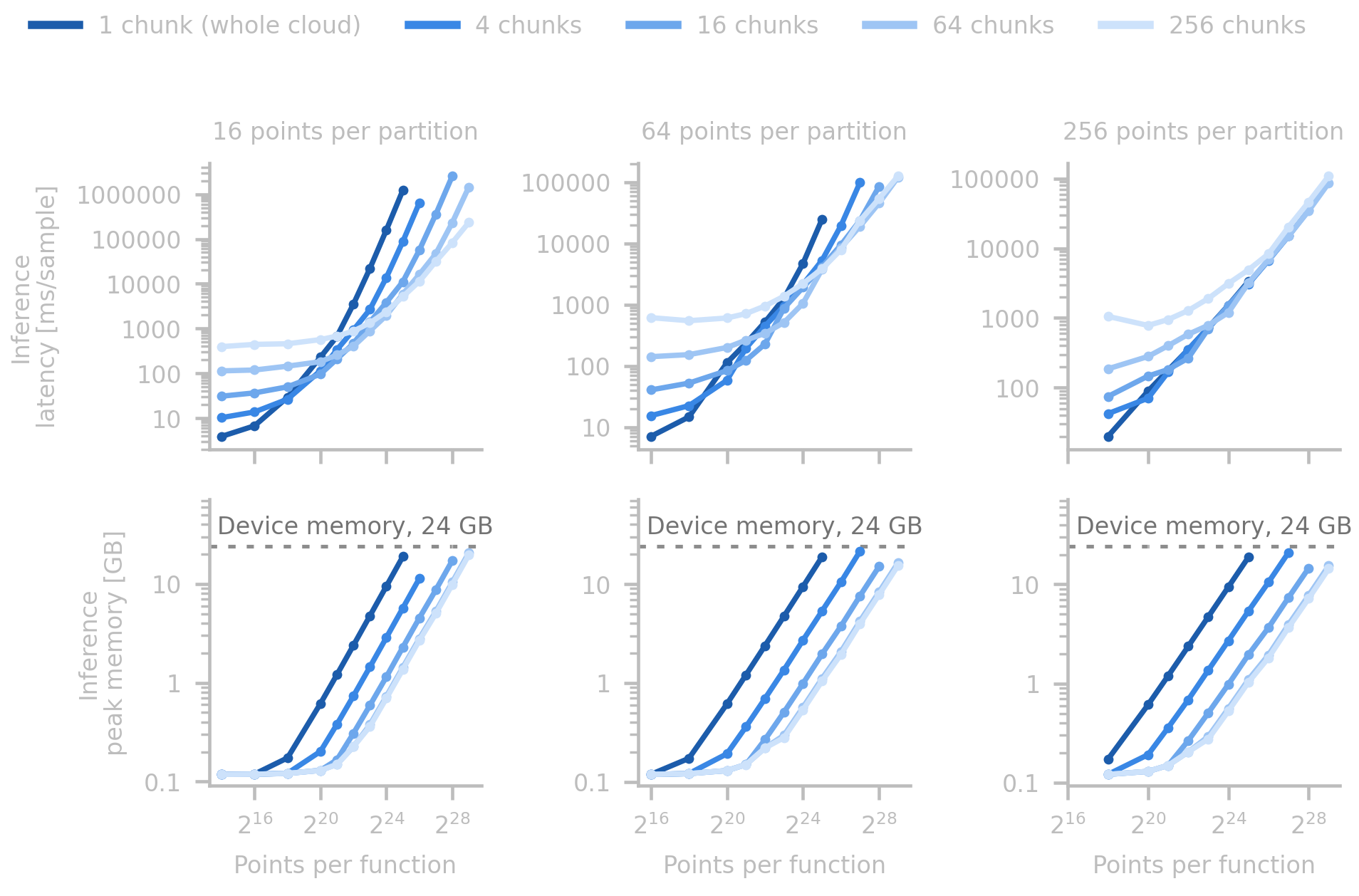
The memory of inference grows linearly with the points, which bounds the size of a function one GPU can map. The encoder reduces every partition on its own and the decoder reads every point from its own coordinate and the embeddings of its partitions, so neither needs the whole cloud at once. Chunked inference cuts the points into chunks of equal size along a space-filling curve, partitions every chunk on its own, and encodes and decodes one chunk at a time, while the processor acts on the embeddings of all chunks together. The mode changes no weight, and a partition never spans two chunks, which changes the result only slightly, from a median relative L² error of 0.208% in one piece to 0.215% in 64 chunks at about a million points.

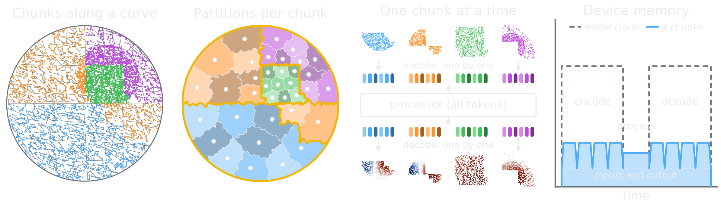
In one piece the largest function that fits on the GPU has 33.6 million points. Sixty-four chunks map 537 million at every density, 16 times more, in 86 seconds within 15.4 GB at 256 points per partition, and at 33.6 million points and 64 points per partition they need 1.1 GB instead of 18.8 GB. On small functions the chunks cost time, since they run one after the other, whereas at 64 points per partition 64 chunks are faster than one piece from about 4 million points, since the cost of the partitioner grows faster than linearly in the partitions it clusters at once. The Inference perks article animates the idea.

The performance figures of the paper

Exploring the latent space

The latent space in which the operators act can be explored directly. The geodesic module on the home page follows an incompressible flow along great circles between anchor embeddings, a zero-shot interpolation in time that drifts off the physical path as the anchors move apart, which is where a learned operator is needed. The interpretability article examines that space in its own right, and the live demos run the analysis backbone on user-provided input, among them the reconstruction of an analytic function, the upsampling of an image and the transition between two fields.