Partitioning

The role of partitions

One embedding per function is a bottleneck, since its size is fixed whether the field is smooth or full of fine structure. Daedalus therefore decomposes the domain. A partitioner splits the N points into P partitions, the same encoder is applied to every partition independently, and a query coordinate is answered from the embeddings of the partitions that cover it. More partitions mean smaller neighborhoods and a finer latent resolution, so P sets the fidelity of the representation, and the benefit of a smaller partition is quantified by its effective spatial frequency.

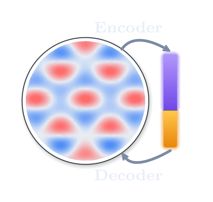
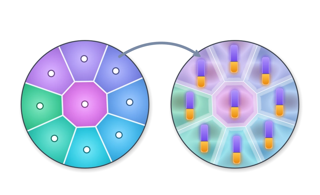
The decomposition turns an unfamiliar global field into a collection of local ones, each of which is simple once it is carried into its own frame, and it lets the cost of the representation follow the content of the field rather than a size fixed in training. The partitions are recomputed for every input and depend on the coordinates alone, never on the values, so two fields observed on the same cloud share their partitions.

k-means initialized along a space-filling curve

The partitions are the clusters of a k-means clustering of the coordinates, computed anew for every input, so the partitioner has to stay cheap on dense clouds and at large partition counts. Lloyd's algorithm starts from the means of P equal runs of the points along a space-filling curve. These initial centers already follow the density of the cloud and induce balanced clusters, so a few iterations reach what many reach from random points, and five are run at inference.

The points are rotated by a random angle, quantized on a grid and sorted by the Morton code that interleaves the bits of their two grid indices, which orders them along a Z-order curve. Within an iteration a point is compared only with the 16 centers nearest to its current one, since the centers move little from one iteration to the next, so the cost of an iteration does not grow with the partition count. The final assignment walks every point from its last center to ever nearer neighboring centers until none is nearer, which recovered the exact nearest center on every cloud tested, and the center of a partition is then recomputed once as the mean of the points nearest to it. Distances are evaluated over chunks of at most 2²⁴ point-to-center pairs, so the full N × P distance matrix is never formed and the memory grows linearly with the number of points.

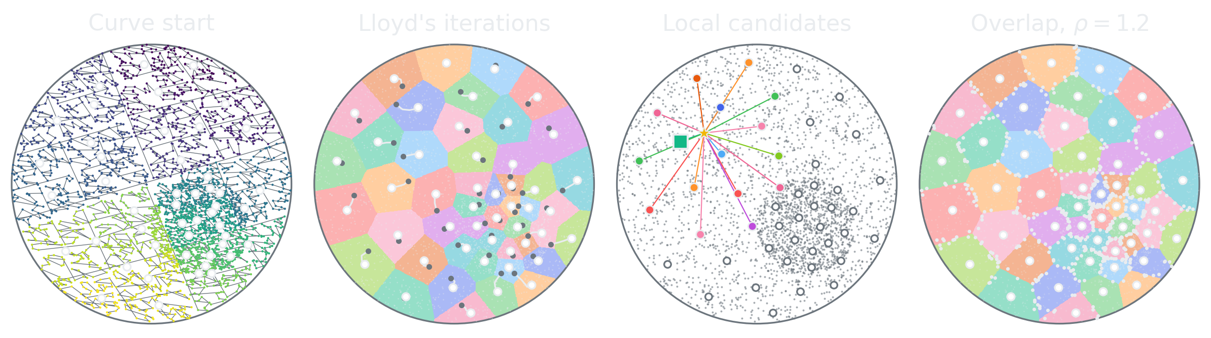
A Morton run is a poor partition in itself, since the curve jumps and a run can consist of two disconnected pieces, but it serves well as an initialization, because the first iteration already assigns every point to its nearest starting center and the subsequent ones refine cells that are close to balanced from the outset.

Overlapping partitions

By default every point belongs to exactly one partition, the one whose center is nearest. An overlap factor ρ ≥ 1 raises the number of point-to-partition assignments to N_asg = ⌊ρN⌋. Every point keeps its own partition, and the further assignments go to the pairs of a point i and a partition p with the smallest distance ratio

r_ip = ‖x_i − c_p‖²min_q ‖x_i − c_q‖² ≥ 1,

ranked over the whole cloud. A ratio near one marks a point almost as close to a neighboring center as to its own, so the surplus extends every partition across its boundary. Since the ranking is global, the further assignments go where partitions are crowded and therefore small, which evens out their sizes. A point in several partitions is decoded by each, and the estimates are averaged. At inference ρ = 1.2, that is, a fifth more assignments than points.

The ranking does not score every pair. A point's further partitions are its second or third choices, so its candidates are the 16 partitions whose centers lie nearest to its own center, and only its 8 best-ranked candidates enter the global ranking, which therefore never scores all NP pairs.

An interactive partitioner

The widget below runs these steps on 3000 points and a selectable partition count.

Partitioning complex domains

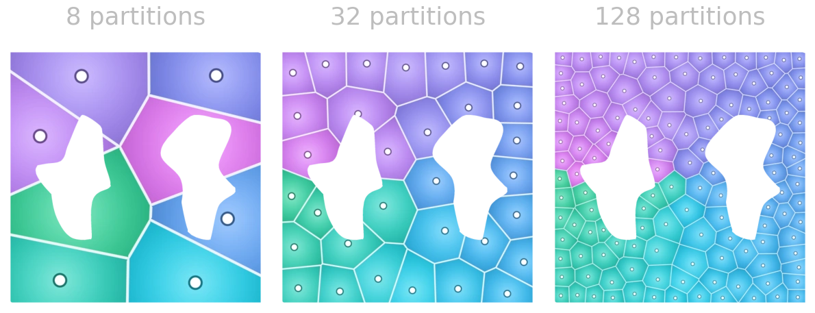
The partitioner requires only the coordinates and therefore applies to any domain on which points can be placed, such as a disk, a square grid of pixels or the point cloud of an elastic body with holes. Whatever the complexity of the domain, the decomposition produces small pieces, and a small piece of a non-convex domain is nearly convex.

The partition count at inference

Since the partitions are recomputed for every input, the partition count is a choice made at inference, not a property of the trained model. In every case the paper examines, more partitions lower the reconstruction error, because every partition then holds less of the variation of the field. The count is bounded in two respects. A partition needs enough points to be represented, so a fixed cloud can be cut only so finely, and a field whose features are finer than its sampling cannot be recovered at any count. For problems too large for one device, the cloud can moreover be cut into independent chunks along a Morton curve and partitioned, encoded and decoded one chunk at a time; this chunked mode of inference, with its measured cost, is the subject of the article on inference perks.

The game Divide and Conquer turns this control into a puzzle. For each of twenty fields, the task is to name the smallest partition count at which the backbone reconstructs the field within 1%, and the error curve of the field against the partition count follows every guess.

Play Divide and Conquer → Read about the inference perks →