Measuring the difficulty of a field
The partition sweeps of the paper show a regularity. Whatever the origin of a field, more partitions improve its reconstruction, and a field that is hard to reconstruct at one partition count becomes easy once its partitions are small enough. This raises the question of whether the difficulty of a field can be measured directly, and whether such a measure would distinguish between kinds of functions at all.
The global frequency content of a field is a natural candidate, but it does not reflect what the encoder reads, since the encoder never sees the global field. Every partition is carried into a common frame, its center moved to the origin, its extent scaled to a box and its values to [−1, 1], and is encoded on its own. What decides how hard a partition is to represent is therefore how much variation remains inside it once it has been normalized. Cutting a field into smaller partitions and rescaling each one leaves less of that variation in every partition, as the first figure of the paper illustrates on one field.
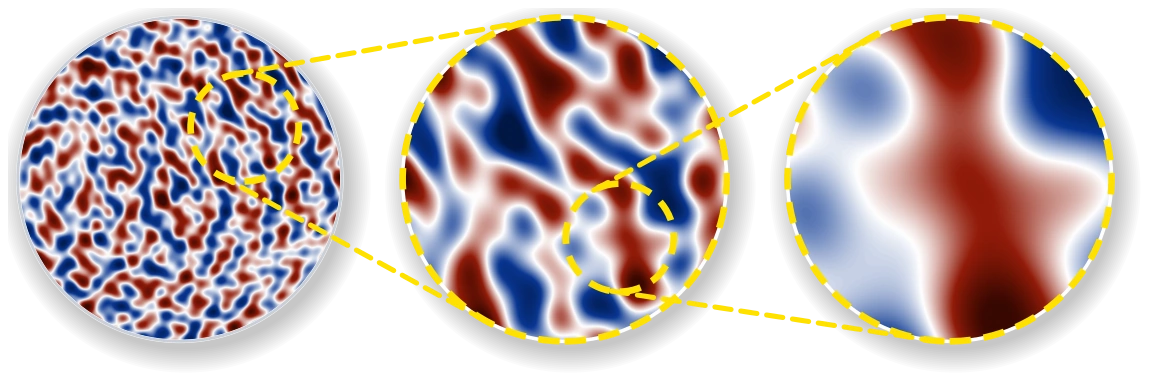
The widget below reproduces this effect on three fields of different families, radial sines of frequency 7, narrow Gaussian bumps and plane waves of low frequency. Drag the yellow window over the field and set its magnification. The window is shown as the encoder would read it, its center at the origin, its extent scaled to the unit disk and its values mapped onto [−1, 1], and its effective frequency, defined below, is updated as the window moves. The gauge places it on the distribution of the training functions.
Definition
The coordinate frame of a partition p maps its region Ωp onto a region Ω̃p inside the box [−1, 1]2, by moving its center cp to the origin and dividing every axis by the partition's extent sp along it. By the chain rule, the gradient and the Hessian of the field with respect to these normalized coordinates are ∇x̃u = sp ⊙ ∇u and ∇2x̃u = (spsp⊤) ⊙ ∇2u, with ⊙ the elementwise product. The effective spatial frequency (ESF) of the partition is the Rayleigh quotient of the second derivatives over the first,
feff,p = 12π (∫Ω̃p ‖∇2x̃u‖F2 dx̃∫Ω̃p ‖∇x̃u‖22 dx̃)1/2.
It measures how quickly the slope of the normalized field changes across the partition, relative to the slope itself. Three properties make it depend on the normalized partition that the encoder reads, and on nothing else.
- The value frame drops out. The value shift of a partition has no derivative, and its value scale multiplies both integrals by its square, so normalizing the values does not change feff,p.
- The size drops out. The derivatives are taken in the normalized coordinates, so a feature of a given shape has the same feff,p whether it fills a large partition or a small one.
- An affine field has frequency zero. A partition on which the field is affine has no second derivatives. Its normalized field is a ramp, which carries no information beyond its direction.
Calibration on a plane sine
The factor 1/2π calibrates the quotient so that it recovers the frequency of a single sine. Take one partition that covers the unit disk, which is its own normalized frame, and the sine u(x) = a sin φ(x) of frequency f, with the phase φ(x) = 2πf n·x + φ0 along a unit direction n. Its gradient is 2πf a cos φ n and its Hessian −(2πf)2a sin φ nn⊤, a matrix of unit Frobenius norm times a scalar, so
feff,p = f (∫ sin2φ dx∫ cos2φ dx)1/2.
Over a region that holds whole periods along n, the two integrals are equal and feff,p = f exactly. The ESF is therefore expressed in the same units as the frequency of a sine.
Aggregation over the partitions of a field
A field cut into partitions has one ESF per partition, but its reconstruction error is measured on the whole field, so relating the two requires one frequency for the whole field, which follows from how the partitions share the variation of the field. For disjoint partitions, with ū the mean of the field over the domain and ūp its mean over partition p, the energy of the centered field splits exactly into two parts,
‖u − ū‖2L2(Ω) = ∑p ‖u − ūp‖2L2(Ωp) + ∑p |Ωp| (ūp − ū)2,
because the field minus its partition mean integrates to zero over every partition, so the cross terms vanish. The first sum is the variation inside the partitions, which the embeddings have to represent. The second is the variation between the partition means, which the frames carry exactly through their value shifts. With ωp the share of the energy of the centered field that lies inside partition p, and the remaining share ω0, that of the frames, counted at frequency zero, the ESF of the partitioned field is the root mean square
feff = (∑p ωp feff,p2 + ω0·0)1/2, ωp = ‖u − ūp‖2L2(Ωp)‖u − ū‖2L2(Ω).
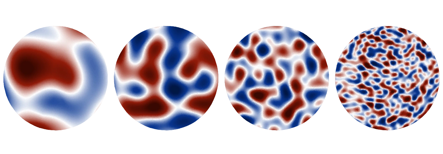
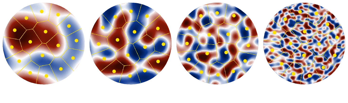
On a single partition ω1 = 1 and feff is the ESF of that partition. As the partitions shrink, two effects lower feff, since every partition holds fewer oscillations and more of the variation moves into the frames, which count at zero.
Choice of the weights
The weights are those with which the partitions enter the error of the whole field. Write û for the reconstruction and ep = ‖û − u‖L2(Ωp) / ‖u − ūp‖L2(Ωp) for the relative error of partition p. For disjoint partitions, exactly,
‖û − u‖2L2(Ω)‖u − ū‖2L2(Ω) = ∑p ωp ep2.
The frame of a partition is replayed exactly, so its reconstruction error is its value scale times the error of its normalized decode, and ep does not depend on the frame: like feff,p, it is a property of the normalized partition. The variation between the partition means is reproduced by the frames and adds no error. The squared error of the field is therefore the average of the squared errors of the partitions with the weights ωp, with zero weight on the share of the frames, and feff averages their frequencies in the same way. A plain mean or median over the partitions would instead weigh a nearly flat partition, which contributes almost nothing to the error, as heavily as one that holds most of the variation of the field, and would ignore that a field whose variation lies mostly between its partitions is reproduced by the frames.
The same identity determines which error to relate to feff, namely the error relative to the centered field. A constant offset of a field is carried by the frames exactly, so the usual relative error, divided by the norm of the field itself, would call a field with a large offset accurate whatever its shape. The measurement below therefore uses the centered error, unlike every other measurement of the paper.
An interactive example
The widget below computes both quantities for a field of three isotropic radial-sine modes of one frequency, with the partitions of the inference partitioner.
Measurement protocol
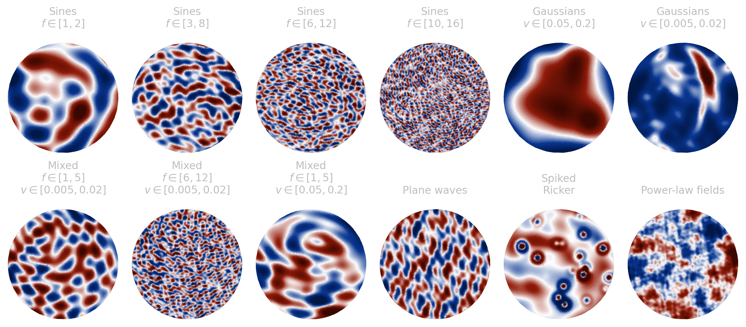
The measurement tests whether the reconstruction error of the analysis backbone depends on feff alone, on twelve synthetic families, chosen to differ in kind rather than only in parameters:
- radial sines of 25 modes with frequencies in [1, 2], [3, 8], [6, 12] and [10, 16];
- Gaussian bumps of 100 modes, wide and narrow;
- three equal mixtures of bumps with radial sines, the narrow bumps with sines in [1, 5] or [6, 12] and the wide bumps with sines in [1, 5];
- plane waves of 10 modes with frequencies in [1, 8], straight wavefronts across the whole domain;
- spiked fields, 20 smooth Ricker spikes of width 0.05 on radial sines;
- power-law fields, random fields of 200 modes with the power spectrum |f|−3, whose energy is spread over a whole range of wavenumbers rather than concentrated in a band.
Every family contributes a fixed set of 64 functions, each sampled once at 32,768 points drawn uniformly on the unit disk. At P partitions, from 1 to 128, a function is reconstructed from the first 256P of its points, again a uniform sample of the disk, so a partition holds 256 points on average at every partition count. Holding the points per partition fixed keeps the frequency apart from undersampling, a separate source of error that would otherwise grow with the partition count. The partitioner runs without overlap, which makes the partitions disjoint, as the energy split requires. Every family is given in closed form, so the gradients and Hessians are evaluated exactly at the points, and the integrals become sums over the points of each partition. A point of a curve is the median over the 64 functions of the error of the centered field against the median of their feff, both on the same points and partitions.
The histogram along the frequency axis is the ESF of 1024 functions of the training distribution of the analysis backbone, as the backbone sees them during training.
The effective spatial frequency determines the accuracy
Every family above is reconstructed by the same frozen backbone at 1, 2, 4 and up to 128 partitions, and for every partition count two numbers are recorded, the median error of the reconstruction, measured against the centered field, and the median effective frequency feff of the partitioned field. Each family therefore traces one curve of error against feff. Its right end is the field on a single partition, where feff is highest, and every step to the left doubles the partitions, which lowers feff,p in every partition and with it feff. Only the partition count changes along a curve.
The families were chosen to have little in common: radial waves with curved fronts, straight plane waves, isolated bumps, sharp spikes on a smooth background, and power-law fields whose energy is spread over many scales. Judged by their global appearance or their spectra, they pose very different problems, and their curves nevertheless fall on top of one another. Two fields of different families with the same feff are reconstructed about equally well, and a field that is far from the training distribution as a whole behaves much like a training function once its partitions bring feff down to the same value. Radial sines with frequencies in [3, 8], for example, start at an feff of 5.4 and an error of 88% on one partition and reach 0.45 and 0.76% at 128 partitions, on the same path as the other families.
The shaded bands show where the training functions lie: half of them have an feff below 0.76 and 95% below 1.7. The error is low inside this band and rises steeply above it. Measured in the frame in which the encoder operates, the family a field belongs to has little bearing on how hard it is to represent, and one number of the normalized partitions largely fixes the error. This is what makes a backbone trained on smooth sines alone useful for shocks, stresses and photographs, since their partitions, once small enough, look like the partitions it was trained on.
Implications and limits
Out-of-distribution transfer is, in these terms, not extrapolation. An unfamiliar global field is decomposed into partitions whose effective frequency the model has seen, and the partition count becomes an accuracy control set at inference, per input and per task, without retraining.
The same statement also sets the limit of the approach. What bounds the representation is a frequency band fixed by the training distribution, and a partition whose ESF lies outside that band is not represented accurately, however the rest of the domain is partitioned. How finely a field can be partitioned is in turn bounded by its sampling, since a partition needs enough points to be represented. Overlapping partitions reuse points and relax this bound, but each partition then covers a larger area and carries a higher effective frequency. Neural operators show the corresponding effect, learning only the frequencies present in their training data, and these measurements locate it one level lower, in the representation of the input itself.
Two games on the effective frequency
Two games build on the effective spatial frequency. Freaks shows fields of radial sines, each with ten modes and its own frequency range, and asks for an estimate of feff of each from its picture alone, scored against its exact value, either as twenty fields in five minutes with the true value after every guess or, in a speed mode, as many hits within a factor of 1.2 as possible in one minute. Divide and Conquer poses the converse problem, the smallest number of partitions with which the backbone reconstructs a field within 1%. A field needs more partitions the higher its ESF, until each partition's ESF falls inside the band the model was trained on, so the first game prepares for the second. Every finished game enters the leaderboard of its game, shown below, under a random nickname.