Partition normalization

Coordinate and value frames

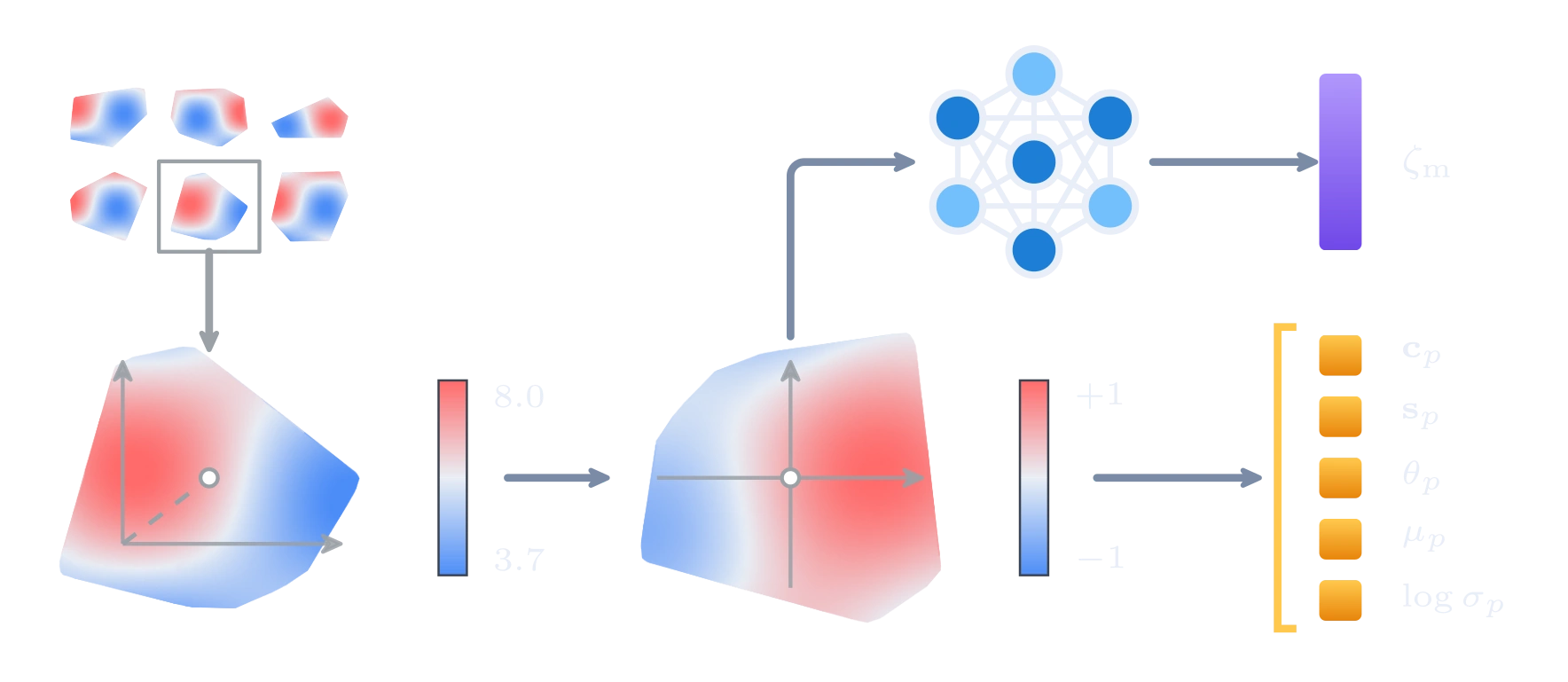
A partition of a field can sit anywhere in the domain, be large or small, stretched along one axis, and carry values of any offset and any range. An encoder that had to model all of this would spend its capacity on the location, size and amplitude of a feature rather than on its shape. PartNorm removes these quantities before the encoding and stores them separately.

Let ℐ_p be the points assigned to partition p and c_p its center. The coordinate frame shifts the points to the center and scales every axis by the largest distance from it,

x̃_i = (x_i − c_p) ⊘ s_p, s_p,d = max_{i∈ℐ_p} |x_i,d − c_p,d|,

with ⊘ the elementwise division, so that every partition fills the box [−1, 1]² whatever its size and shape. The value frame maps the values of the partition onto [−1, 1] through their mid-range and half-range,

ũ_i = (u_i − μ_p) / σ_p, μ_p = ½(max u + min u), σ_p = max{½(max u − min u), σ_min},

with the extrema taken over the partition and a floor σ_min = 10⁻⁸ that keeps the scale positive. The mid-range and the half-range, rather than a mean and a standard deviation, guarantee that every normalized value lies in [−1, 1], the range the decoder is trained to produce.

PartNorm in motion, on a field of three radial-sine modes at 2400 points cut into 8 partitions. One partition at a time is shifted by its center c_p, scaled along every axis by its extent s_p into the box [−1, 1]², and its values are mapped onto [−1, 1] by μ_p and σ_p, so that every partition reaches the encoder at the same position, size and amplitude. The frame is kept as the static features.

Static features

The quantities that define the frame, namely the center, the axis scales, an orientation angle, the value shift and the logarithm of the value scale, (c_p, s_p, θ_p, μ_p, log σ_p), are retained as the static part ζ_s,p of the embedding. The encoder reads only the normalized pairs (x̃_i, ũ_i) and returns the morphologic part ζ_m,p, which describes only the normalized shape of the partition. The embedding of a partition is the pair ζ_p = (ζ_s,p, ζ_m,p). The value scale is stored as a logarithm, so that a processor which predicts it works on a quantity of moderate range whatever the amplitude of the field.

One partition out of six is shifted and scaled into a centered frame, its values mapped from their own range to the range from minus one to one, and encoded into a morphologic embedding beside five static features — PartNorm (panel c of the overview figure). A partition is shifted to its center and scaled into the box [−1, 1]², its values are mapped from their own range onto [−1, 1], the encoder turns the normalized partition into the morphologic embedding ζ_m, and the five quantities of the frame are kept as the static features ζ_s. The trained backbones fix the angle at zero.

The widget below computes this frame for a field of three radial-sine modes at 8192 points cut by the inference partitioner, without overlap.

PartNorm of one field. Left, the field in a common color scale with the selected partition highlighted, its center (white) and the box [c_p − s_p, c_p + s_p] that the frame maps onto [−1, 1]² (dashed). Right, the same partition in its frame, colored on the fixed scale [−1, 1], with the points the encoder receives (small dots). The list gives the static features and the effective spatial frequency of the partition.

Degenerate partitions

Two degenerate cases are treated separately. An empty partition has no extrema and receives μ_p = 0 and σ_p = 1. A constant partition has a mid-range but no range, and only its scale is raised to the floor, so it decodes to μ_p up to a term of order σ_min, and the constant is reproduced to floating-point precision whatever the network returns.

Canonical rotation

The encoder can optionally rotate every partition into a canonical orientation, by an angle read from the dipole or the quadrupole moment of its normalized values, and the decoder replays it. The trained backbones do not apply this rotation, so θ_p = 0 and the orientation of a partition stays in its morphologic embedding, since the encode-decode map is approximately equivariant to rotation without it. The rotation can nonetheless be switched on at inference with the trained weights unchanged. The decoder replays the stored angle, so encoding and decoding stay exact and the reconstruction is essentially unaffected, and rotated copies of one partition then map to the same morphologic embedding.

Coincidence of similar partitions Read more about the effective spatial frequency →

Normalization carries structurally similar partitions to nearly identical inputs, whatever their global context, so their embeddings coincide. A high-frequency field observed in a small partition normalizes to almost the same input as a low-frequency field in a large one, because within a partition absolute scale is immaterial and only the number of oscillations across the partition survives. The model therefore needs to have seen partitions of comparable normalized morphology rather than fields of the same physical type, which is what the effective spatial frequency measures.

The figure below follows three pairs of inputs through the frame, each partition encoded as a single partition by the analysis backbone, with the optional rotation switched on so that a rotated input lands in the same orientation. Each pair tests one property, quantified by the cosine similarity of the two morphologic embeddings ζ_m^A and ζ_m^B.

Input A on the unit disk with its partition circled — PartNorm on three pairs of inputs (the paper's appendix figure, one pair at a time). Each input is drawn in a colormap of its own, except the pair of one function, which shares one colormap and one range so that B's larger values show; its partition is circled. The normalized partitions are drawn in the canonical frame on [−1, 1], with their static frames: the largest axis scale s_p, the angle θ_p of the canonical rotation, the value shift μ_p and the value scale σ_p. The strip shows the 128 components of the two morphologic embeddings and the magnitude of their difference; hover over a cell to read it.

The partition of input A in the canonical frame — PartNorm on three pairs of inputs (the paper's appendix figure, one pair at a time). Each input is drawn in a colormap of its own, except the pair of one function, which shares one colormap and one range so that B's larger values show; its partition is circled. The normalized partitions are drawn in the canonical frame on [−1, 1], with their static frames: the largest axis scale s_p, the angle θ_p of the canonical rotation, the value shift μ_p and the value scale σ_p. The strip shows the 128 components of the two morphologic embeddings and the magnitude of their difference; hover over a cell to read it.

In the first pair, input B oscillates three times faster than input A and is also rotated, rescaled and shifted in its values, and its partition is three times smaller. Each of these differences is a transformation the frame removes, and all of them are absorbed by the static features, which differ widely (B's scale is a third of A's, its value scale nearly three times larger). The normalized partitions coincide, and so do the embeddings, with a cosine similarity of 99.7%.

The second pair distinguishes what the frame removes from what it does not. The two inputs are one function on partitions of the same size, B being A scaled by 1.5 and shifted by 2.5, so that on one color scale they take its opposite ends, but B's value scale and shift also vary mildly across the partition. The frame removes one value shift and one value scale per partition, which absorbs the difference of the two frames entirely, as μ_p and σ_p show. The variation across the partition is not a transformation of the whole partition, so it survives into the normalized values, and the embeddings agree closely but not exactly, with a cosine similarity of 89.7%. A heterogeneous frame is therefore normalized away only to the extent that it is constant over a partition, and a finer partition, over which it varies less, removes more of it.

In the third pair the inputs are two independent functions of different morphologies. Their normalized partitions stay different, and so do their embeddings, with a cosine similarity of 69.7%. Normalization therefore identifies partitions that differ only by the transformations it removes, and keeps apart partitions that differ in their morphology, so one encoder serves fields of any location, size and amplitude without conflating fields of different shape.

The factorization extends the shape-gain decomposition of the Phaedra tokenizer, which separates the shape of a feature from its magnitude on a regular grid, to a full local frame on every partition of an arbitrary cloud.

Restoring the frame at decoding

The decoder replays the frame, evaluating the normalized field at the frame coordinates of a query point and mapping it back through the value frame, and a point that lies in several partitions averages their estimates,

u(x) ≈ 1|𝒜(x)| ∑_p∈𝒜(x) ( μ_p + σ_p 𝒟( ζ_m,p, (x − c_p) ⊘ s_p ) ),

with 𝒜(x) the partitions that contain x. Since the frame is replayed exactly, the error of encoding and decoding a partition is the error of the normalized decode multiplied by σ_p. A partition whose values barely vary therefore contributes almost no error, whatever its offset, and the error of a field concentrates in the partitions that hold most of its variation.

Equivariance by construction

The frame makes the encode-decode map, which encodes a field and decodes it again, equivariant to the transformations it normalizes away. A translation or a dilation moves the centers and the extents of the partitions with the points, c_p ↦ sc_p + c and s_p ↦ ss_p, for a translation c and a dilation s, and leaves the normalized coordinates unchanged. A shift or a positive scale of the values moves the mid-range and the half-range, μ_p ↦ σμ_p + μ and σ_p ↦ σσ_p, for a value scale σ > 0 and a value shift μ, and leaves the normalized values unchanged. The encoder reads only the normalized pairs, so the morphologic embedding is invariant to all four transformations, the static features take them up, and the decoder, which replays them, returns the transformed reconstruction. The equivariance is exact and holds by construction on an unstructured cloud, and no latent capacity is spent on the location, size or amplitude of a feature.

The paper measures this on the analysis backbone, over translations up to 100 disk radii, dilations between 1/100 and 100, value shifts up to ±1000 times the root mean square of the field, and value scales between 1/1000 and 1000. Over all four ranges the error of the transformed field does not change, and the equivariance error, the distance between the reconstruction of the transformed field and the transformed reconstruction stays well below the reconstruction error. Rotation, which the backbones do not normalize, changes the embeddings, yet over a full turn the error does not change and the equivariance error stays below the reconstruction error.

error, transformed fieldequivariance error, partitions carriedequivariance error, partitions recomputed (translation, dilation, rotation)

Equivariance of the encode-decode map, one transformation at a time. For each transformation, the relative L² error of the reconstructed transformed field, and the equivariance error, the distance between the reconstruction of the transformed field and the transformed reconstruction, with the partitions carried along with the transformation and recomputed on the transformed cloud. Analysis backbone, 16 functions with three radial-sine modes of frequencies in [1, 4], at 8192 points and 64 partitions.

When the partitions are recomputed on the transformed cloud instead of carried along, the partitioner's random curve and its finite iterations give slightly different cells, and the equivariance error then measures how much the reconstruction depends on where the cells fall. It stays below the reconstruction error as well.