Physical fields from nine datasets
The paper tests the analysis backbone on ten fields from real datasets, seven fields on regular grids, of compressible flow with shocks and shear layers, of an acoustic wave and of an incompressible flow, encoded with 1024 partitions, and three fields of elastic bodies on point clouds with holes, encoded with 128 partitions. None of these fields is a radial sine or is defined on a disk, and the domains of the elastic bodies are not convex. The reconstructions recover fine texture in addition to the coarse layout.
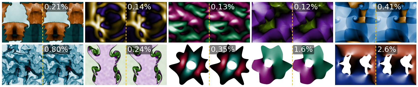
The geometry of a domain reaches the backbone only through the partitioner. A grid of pixels, a disk and the point cloud of a body with holes are all cut into small partitions, each of which is close to convex in its own frame, so an unseen domain poses no difficulty of its own. The accuracy is governed by the variation of the field within each partition, which is independent of the global domain.
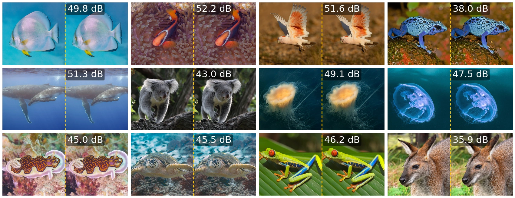
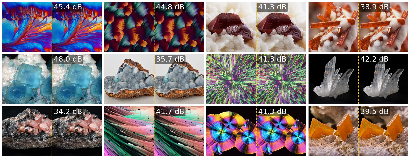
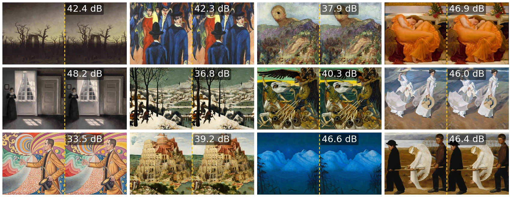
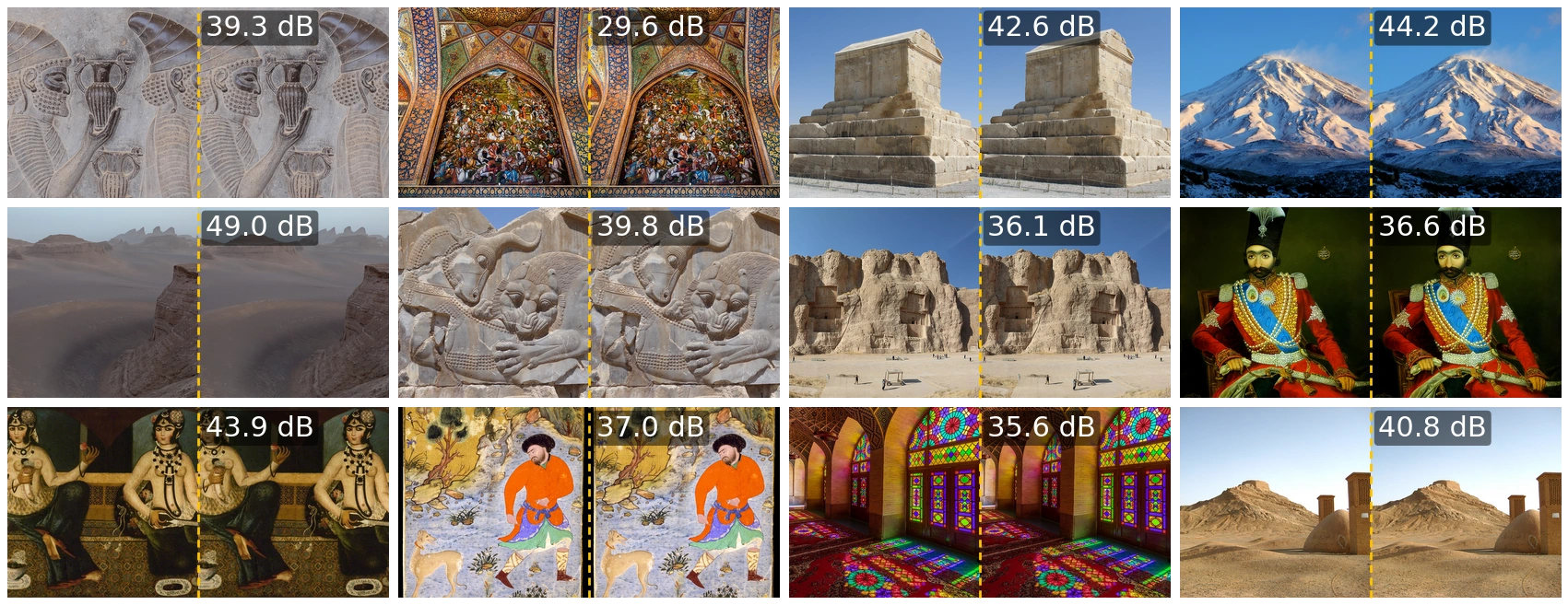
Every input under a before-and-after slider: drag across a panel, or move the divider with the arrow keys, to compare the input (left) with its reconstruction (right), and change the number of partitions, from 1 to 1024, to follow how detail is resolved. Errors are measured at the input points. The elasticity field on its point cloud has 10,000 points and is shown with at most 128 partitions. Photographs from Wikimedia Commons; credits.
Photographs
A photograph is three scalar functions on a pixel grid, and the frozen model encodes each color channel like any other input. The paper reconstructs 48 photographs in four groups, animals, minerals and crystals, paintings, and Persian art and places, most of them Featured Pictures of Wikimedia Commons. Each is cut to its central square, resampled to 512 × 512 pixels and reconstructed with 4096 partitions per channel, about 64 pixels per partition, and the median peak signal-to-noise ratio (PSNR) is 42.3 dB, with a range from 29.6 to 52.3 dB. The lowest values belong to texture finer than a partition, such as a densely painted fresco, a pointillist painting or rhodochrosite crystals on a granular rock, and the highest to content dominated by smooth regions, such as whales in open water or a clownfish before a blurred anemone.
The partition count as a resolution
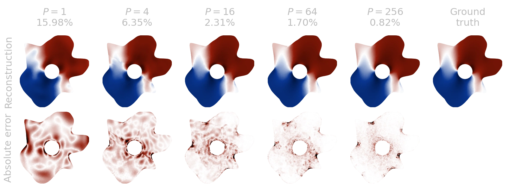
The partition count is the resolution control of the representation. In every case examined in the paper, the error decreases steadily as the count grows. For the Cauchy stress σyy of a hyperelastic body on a domain with a hole it falls from 16.0% with a single partition to 0.82% with 256. The error concentrates around the hole and at the corners of the boundary, where the stress varies fastest, and recedes there as the partitions shrink. An incompressible-flow velocity follows the same course, from 36.3% with one partition to 0.18% with 256.
Points required per partition
The partition count fixes how many embeddings describe a field, and the input resolution how many points each embedding is computed from. Growing the partition count on a fixed cloud eventually starves every partition of points. Scored at points the encoder did not see, on a cloud of 8192 points, the error is lowest at 64 partitions of 128 points and grows almost fivefold by 512 partitions of 16 points. At the encoded points themselves the error would continue to fall, since an embedding can store the few values it receives, and the loss of accuracy is visible only at held-out points. Growing the cloud with the partition count keeps the points per partition constant, and the held-out error then keeps falling at every density tried, from 16 to 128 points per partition, to between 1.34% and 0.10% at 2048 partitions, the denser partitions lower throughout. More partitions therefore cost accuracy only when they leave too few points in each.
The widget below shows one function of that experiment, decoded at the pixels of the disk, none of which the encoder saw.
Functions on curves
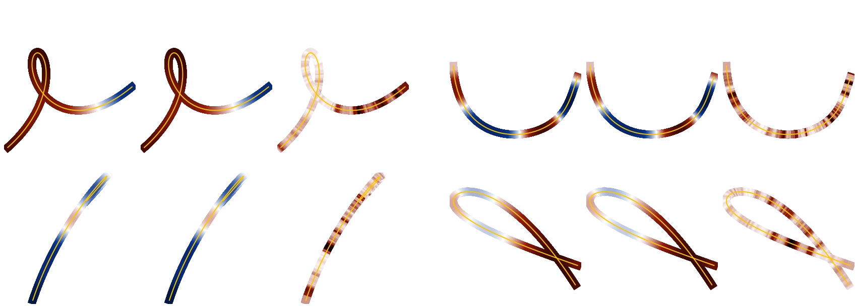
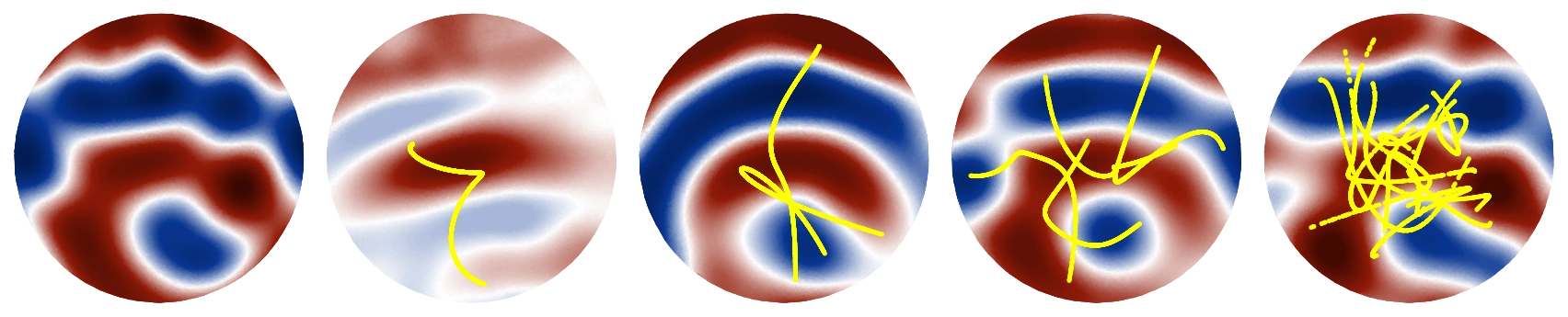
The encoder aggregates whatever points a partition holds, so a partition that contains only a piece of a curve is as admissible an input as one that fills an area. Although trained only on functions that fill a disk, the same model accepts a function sampled on a one-dimensional curve in the plane, such as a boundary trace. Encoded with 16 partitions and decoded on the same points, the reconstruction follows the observed values along each curve with a small, unstructured error.
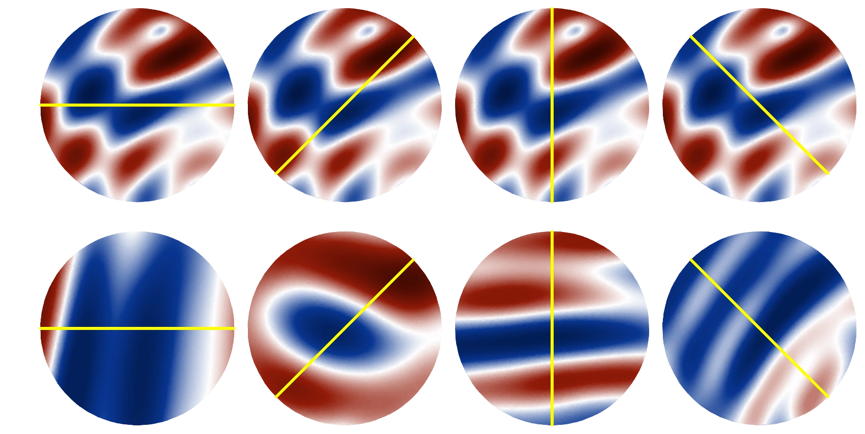
A curve under-determines the field around it, yet the decoder, which can be queried anywhere, returns a two-dimensional function. Observed on a straight line through the disk, a field is tracked along the line, while off the line the decoder returns a plausible smooth continuation that the observation does not constrain, a different one for every direction of the line. Different curves through one field likewise give different plausible completions, which indicates that the encoder does not return a memorized training function, and as more curves cover the domain the observations constrain more of it and the true field re-emerges. A latent space shared by functions on a domain and on its boundary serves operators whose inputs and outputs live on sets of different dimension, since boundary data then arrive already extended into the interior.

Partial observations
Two experiments on a single partition probe partial observation from opposite sides, for radial-sine fields with 1 to 10 modes in the training band and a mask at radius 0.5. Observing only the inner disk and decoding on the whole disk, the observed region is reconstructed to below 1%, the continuation stays at about 5% in the band 0.5 < r < 0.6, and it becomes unconstrained further out, reaching 44 to 77% in the outermost band. Observing only the annulus 0.5 < r < 1 instead, the inner disk is filled in, an inpainting task, to about 2% for one or two radial modes, and the error grows to about 20% for five and ten modes, as the unobserved region becomes increasingly under-determined.
Where an observation leaves part of a field unconstrained, the completion resembles the training functions, a smooth field off a curve and radial wavefronts beyond an observed disk. This bias is a property of the training distribution rather than of the architecture. A backbone trained on another family of functions would complete an unobserved region with functions of that family, so the training distribution acts as the prior of every partially observed reconstruction and should match the structure an application expects where it observes nothing.
Two live demos apply the same single-partition completion to inputs of one's own choosing. The inpainting demo hides holes in a field or a picture, painted by hand or taken from a set of preset masks, and fills them from the embedding of the observed rest. The outpainting demo observes only a window, of adjustable shape and position, and continues the field from it over the whole disk.